Different Information Scenarios in maxent_disaggregation#
This notebook demonstrates how the sampling behavior of maxent_disagg() changes based on the information you provide.
The maxent_disagg() function internally handles two key aspects:
Sampling share distributions (how the total is divided)
Sampling aggregate distributions (the total value)
The package uses decision trees to automatically select appropriate probability distributions based on available information:
For the aggregate value: The distribution choice depends on whether you provide mean, standard deviation, minimum, and maximum bounds.
For the shares: The distribution choice depends on whether you provide best estimates and standard deviations.
# Import necessary libraries
import numpy as np
import matplotlib.pyplot as plt
from maxent_disaggregation import maxent_disagg, plot_samples_hist, sample_aggregate, sample_shares

# Set sample size for demonstrations
N = 10000
Sampling Shares#
The maxent_disagg() function samples the relative proportions that must sum to 1. The sampling method depends on what information you provide.
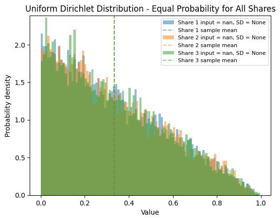
Uniform Dirichlet Distribution#
When no information about shares is available (using np.nan), the function uses a uniform Dirichlet distribution where all components are equally likely.
# Define shares with no information
shares_disaggregates = [np.nan, np.nan, np.nan]

# Sample using maxent_disagg
samples, _ = sample_shares(n=N,
                           shares=shares_disaggregates)

# Plot the results
plot_samples_hist(samples, shares=shares_disaggregates,
                  plot_agg=False,
                  title="Uniform Dirichlet Distribution - Equal Probability for All Shares")
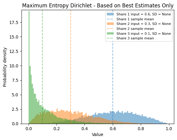
Maximum Entropy Dirichlet Distribution#
When you provide best estimates for the shares but no uncertainty information, maxent_disagg() uses a Maximum Entropy Dirichlet distribution.
# Define shares with best estimates
shares_disaggregates = [0.6, 0.3, 0.1]

# Sample using maxent_disagg
samples, _ = sample_shares(n=N,
                           shares=shares_disaggregates)

# Plot the results
plot_samples_hist(samples, shares=shares_disaggregates,
                  plot_agg=False,
                  title="Maximum Entropy Dirichlet - Based on Best Estimates Only")
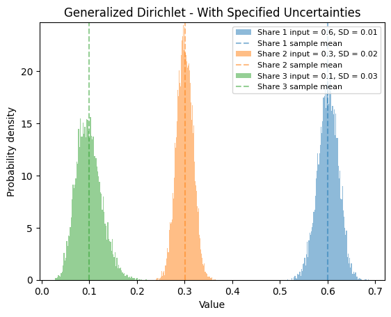
Generalized Dirichlet Distribution#
When you provide both best estimates and standard deviations for the shares, maxent_disagg() uses a generalized Dirichlet distribution.
# Define shares with best estimates and standard deviations
shares_disaggregates = [0.6, 0.3, 0.1]
sds_shares = [0.01, 0.02, 0.03]

# Sample using maxent_disagg
samples, _ = sample_shares(n=N,
                           shares=shares_disaggregates,
                           sds=sds_shares)

# Plot the results
plot_samples_hist(samples, shares=shares_disaggregates,
                  sds=sds_shares,
                  plot_agg=False,
                  title="Generalized Dirichlet - With Specified Uncertainties")
Sds above threshold: [1.18506436], sds: [0.01], sample_sd: [0.02185064], indices: [0]
/Users/ajakobs/Documents/code_projects/maxent_disaggregation/maxent_disaggregation/shares.py:475: UserWarning: The generated samples for the shares have a standard deviation that is more than 20.0% different from the specified sd's. Please note that the specified sd's might be incompetibale with the other constraints. Please check your inputs. To surpress this warning you can set a higher threshold_sd.
  warnings.warn(
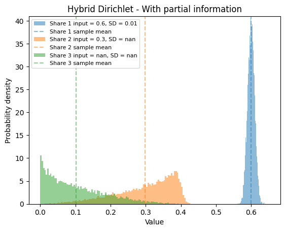
Hybrid Dirichlet Distribution#
When you provide partial information on the best estimates and standard deviations for the shares, maxent_disagg() uses a hybrid sampling using Beta- and Maximum Entropy Dirichlet- distributions.
# Define shares with best estimates and standard deviations
shares_disaggregates = [0.6, 0.3, np.nan]
sds_shares = [0.01, np.nan, np.nan]

# Sample using maxent_disagg
samples, _ = sample_shares(n=N,
                           shares=shares_disaggregates,
                           sds=sds_shares)

# Plot the results
plot_samples_hist(samples, shares=shares_disaggregates,
                  sds=sds_shares,
                  plot_agg=False,
                  title="Hybrid Dirichlet - With partial information")
Sampling the Aggregate#
The maxent_disagg() function samples the total value to be disaggregated. Different distributions are chosen based on available information.
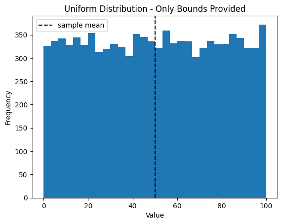
Uniform Distribution#
When only minimum and maximum bounds are provided:
# Sample aggregate using uniform distribution
sample = sample_aggregate(n=N,
                           low_bound=0,
                           high_bound=100,)

# Plot the results
plt.hist(sample, bins=30)
plt.axvline(sample.mean(), ls='--', color='k', label="sample mean")
plt.title("Uniform Distribution - Only Bounds Provided")
plt.xlabel("Value")
plt.ylabel("Frequency")
plt.legend()
plt.show()
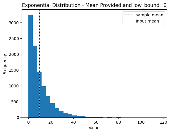
Exponential Distribution#
When a mean but no standard deviation are provided and the low_bound = 0 and upper_bound=np.inf or None
# Sample aggregate using exponential distribution
sample = sample_aggregate(n=N,
                          mean=10,
                          low_bound=0,
                          )
# Plot the results
plt.hist(sample, bins=30)
plt.axvline(sample.mean(), ls='--', color='k', label="sample mean")
plt.axvline(10, ls=':', color='orange', label='Input mean')
plt.title("Exponential Distribution - Mean Provided and low_bound=0")
plt.xlabel("Value")
plt.ylabel("Frequency")
plt.legend()
plt.show()
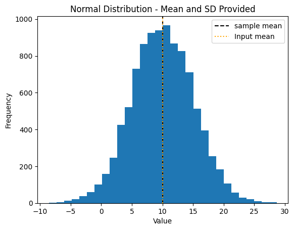
Normal Distribution#
When a mean and standard deviation are provided:
# Sample aggregate using normal distribution
sample = sample_aggregate(n=N,
                          mean=10,
                          sd = 5,
                          low_bound=-np.inf, # default is 0 so set to -inf or None to use normal distribution
                          )

# Plot the results
plt.hist(sample, bins=30)
plt.axvline(sample.mean(), ls='--', color='k', label="sample mean")
plt.axvline(10, ls=':', color='orange', label='Input mean')
plt.title("Normal Distribution - Mean and SD Provided")
plt.xlabel("Value")
plt.ylabel("Frequency")
plt.legend()
plt.show()
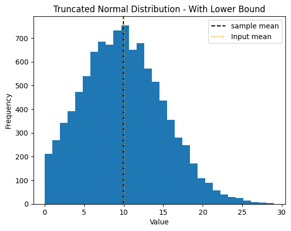
Truncated Normal Distribution#
For non-negative variables, you can set a lower bound of zero. For general bounds \([a,b]\) you can set the low_bound and high_bound to \(a\) and \(b\) resepctively. The truncated normal distribution is the MaxEnt solution for a known best guess and standard deviation on a bound interval. To use the truncated normal please set log=False.
For bounds \([0,\infty)\), an alternative often used in Industrial Ecology is to use the lognormal. (The lognormal is the MaxEnt solution when the mean and standard deviation of rhe natural logarithm of the random variable are known.) To use the lognormal distribution set log=True (this is the default for maxent_disaggregation). Please Note that the boundaries of the lognormal are always \([a,b) \equiv [0,\infty)\). If other bounds are given these are set to \([0,\infty)\) and a warning is raised.
# Sample aggregate using truncated normal distribution
mean = 10
sd = 5
low_bound = 0
high_bound = None  # same as np.inf
sample = sample_aggregate(n=N,
                          mean=mean,
                          sd = sd,
                          low_bound=low_bound,
                          high_bound=high_bound,
                          log=False,  # Set to False to sample from the truncated normal distribution
                          )

print(f"Sample mean: {sample.mean()}")
print(f"Input mean: {mean}")
print(f"Sample median: {np.median(sample)}")
print(f"Input bounds: [{low_bound}, {high_bound}]")
print(f"Input Standard Deviation: {sd}")
print(f"sample standard deviation: {sample.std()}")


# Plot the results
plt.hist(sample, bins=30)
plt.axvline(sample.mean(), ls='--', color='k', label="sample mean")
plt.axvline(mean, ls=':', color='orange', label='Input mean')
plt.legend()
plt.title("Truncated Normal Distribution - With Lower Bound")
plt.xlabel("Value")
plt.ylabel("Frequency")
plt.show()
Sample mean: 9.956556841161218
Input mean: 10
Sample median: 9.710258424684524
Input bounds: [0, None]
Input Standard Deviation: 5
sample standard deviation: 5.055988114029651
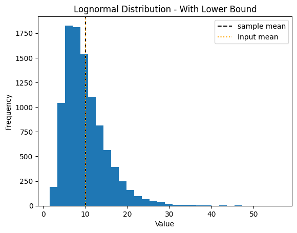
Lognormal Distribution#
An alternative approach for non-negative variables is using a lognormal distribution:
# Sample aggregate using lognormal distribution
mean = 10
sd = 5
low_bound = 0
high_bound = None  # same as np.inf
sample = sample_aggregate(n=N,
                          mean=mean,
                          sd = sd,
                          low_bound=low_bound,
                          high_bound=high_bound,
                          log=True,  # Set to True to sample from the lognormal distribution
                          )

print(f"Sample mean: {sample.mean()}")
print(f"Input mean: {mean}")
print(f"Sample median: {np.median(sample)}")
print(f"Input bounds: [{low_bound}, {high_bound}]")
print(f"Input Standard Deviation: {sd}")
print(f"sample standard deviation: {sample.std()}")

# Plot the results
plt.hist(sample, bins=30)
plt.axvline(sample.mean(), ls='--', color='k', label="sample mean")
plt.axvline(10, ls=':', color='orange', label='Input mean')
plt.legend()
plt.title("Lognormal Distribution - With Lower Bound")
plt.xlabel("Value")
plt.ylabel("Frequency")
plt.show()
Sample mean: 10.050525441884421
Input mean: 10
Sample median: 8.96354983128007
Input bounds: [0, None]
Input Standard Deviation: 5
sample standard deviation: 5.064476353528188
/Users/ajakobs/Documents/code_projects/maxent_disaggregation/maxent_disaggregation/aggregate.py:69: UserWarning: You provided a finite high bound, currently this not supported for the lognormal distribution. High bound is ignored. Alternatively set log=False.
  warnings.warn(
Conclusion#
The maxent_disaggregation package automatically selects appropriate distributions based on the information you provide:
For shares:
No information → Uniform Dirichlet
Best estimates only → Maximum Entropy Dirichlet
Best estimates with SDs → Generalized Dirichlet
For aggregates:
Min/max only → Uniform
Mean/SD only → Normal
Mean with min=0 → Exponential
Mean/SD with min/max → Truncated Normal
Mean/SD with log=True (Default) → Lognormal
This flexibility allows you to incorporate the precise level of information you have available while ensuring statistically valid disaggregation.
a = np.random.rand(10)
b = np.random.rand(10)
c = np.abs(a-b)
d = np.abs(np.log(a/b))
d
array([ 1.38573169,  0.25775963,  0.71622173,  0.41450263,  1.41002268,
        0.21554481,  0.00746703,  0.07712375,  1.17521701, -0.97454063])
np.sqrt((high_bound-mean)*(mean-low_bound))
np.float64(14.142135623730951)