Use Cases and Examples for maxent_disaggregation#
The maxent_disaggregation package enables statistically sound disaggregation of aggregate data with uncertainty propagation. When disaggregating data (splitting a total into components), the components are naturally correlated. These correlations must be properly accounted for in uncertainty analysis to avoid mis-estimating uncertainty in downstream calculations.
This notebook demonstrates how to use maxent_disaggregation through a simple example in Industrial Ecology.
Example: Carbon Footprint of Steel in Vehicle Manufacturing#
Problem Statement#
An Industrial Ecology researcher has data on total steel consumption for vehicle manufacturing but needs to disaggregate this figure by vehicle type (ICE, BEV, and HBEV) based on production volume proxies. A second researcher will use these disaggregated figures for Life Cycle Assessment (LCA).
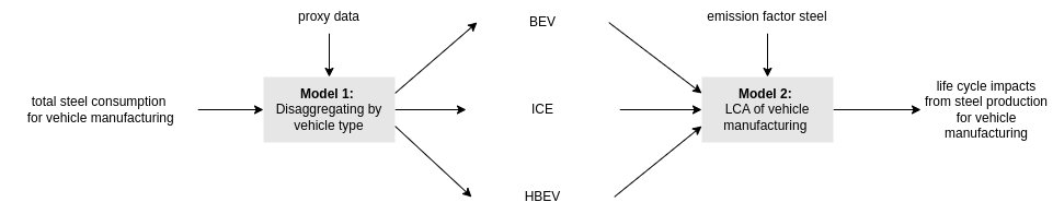
Properly accounting for correlations between the disaggregated values is critical for accurate uncertainty estimation in the LCA.
Available Information#
The first researcher has:
A best estimate for total steel consumption: 100 tonnes/year
An uncertainty estimate for that total: standard deviation of 3 tonnes/year
A natural lower bound of 0 (no negative consumption)
Proxy-based estimates of shares by vehicle type: ICE (80%), BEV (19%), HBEV (1%)
Visualizing the Distribution of Each Component#
# Plot histograms for each vehicle type and the total
plot_samples_hist(
    samples=samples,
    legend_labels=vehicle_types + ['Total'],
    xlabel="Steel Consumption (tonnes)",
    ylabel="Frequency",
    title="Distribution of Steel Consumption by Vehicle Type",
    # ylim= (0, 0.8),  # Uncomment to set y-axis limits, note that this is merely a truncation of the axis and does not change the data
    save=False,
    filename=None
)
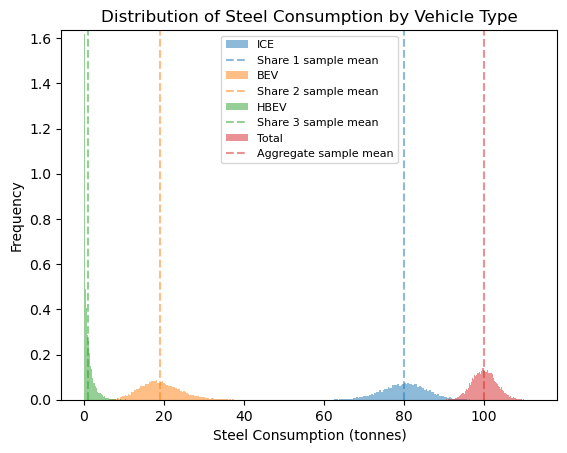
Validating the Samples#
Let’s verify that our samples are consistent with our input information:
# Check if the total matches our specified mean and SD
sample_total = samples.sum(axis=1,keepdims=True)
print("Mean of the sampled total:", sample_total.mean(), "Input total mean:", mean_aggregate)
print("SD of the sampled total:", sample_total.std(), "Input total SD:", sd_aggregate)

# Check if shares match our specified values
sample_shares = np.divide(samples,sample_total)
print("Means of the sampled shares:", sample_shares.mean(axis=0), "Input shares:", np.array(shares))
Mean of the sampled total: 100.02317135623029 Input total mean: 100
SD of the sampled total: 3.0242649175616063 Input total SD: 3
Means of the sampled shares: [0.79916673 0.19084782 0.00998545] Input shares: [0.8  0.19 0.01]
Understanding Correlations in the Sample#
Because the components must sum to the total, they are naturally correlated:
plot_covariances(samples=samples,labels=vehicle_types, title="Covariance of Steel Consumption by Vehicle Type")
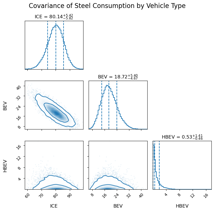
The sign and magnitude of correlations depend on the relative uncertainties of the aggregate and shares. With moderate uncertainty in the total (CV = 3%) and high uncertainty in the shares (default Maximum Entropy behavior, see dirichlet_max_ent for more details), we observe negative correlations between components.
If we increase uncertainty in the total while constraining the shares more tightly:
# Generate correlated samples
samples_2, _ = maxent_disagg(
    n=n_samples,  # Number of samples to generate
    mean_0=mean_aggregate,  # Mean of the aggregate total
    sd_0=50,  # High standard deviation of the aggregate total
    min_0=min_aggregate,  # Lower bound
    shares=shares,  # Best estimates of the shares
    sds=[0.008, 0.0019, 0.0001],  # Very small standard deviations for each share
    log=True,  # Use log-normal distribution for sampling
)

plot_covariances(samples=samples_2,
                 labels=vehicle_types,
                 title="Covariance of Steel Consumption by Vehicle Type \n with High Aggregate SD and low Share SDs")
Sds above threshold: [0.72159933 0.28279297], sds: [0.008 0.0001], sample_sd: [0.00222721 0.00012828], indices: [0 2]
/Users/ajakobs/miniconda3/envs/maxent_disag/lib/python3.14/site-packages/maxent_disaggregation/shares.py:475: UserWarning: The generated samples for the shares have a standard deviation that is more than 20.0% different from the specified sd's. Please note that the specified sd's might be incompetibale with the other constraints. Please check your inputs. To surpress this warning you can set a higher threshold_sd.
  warnings.warn(
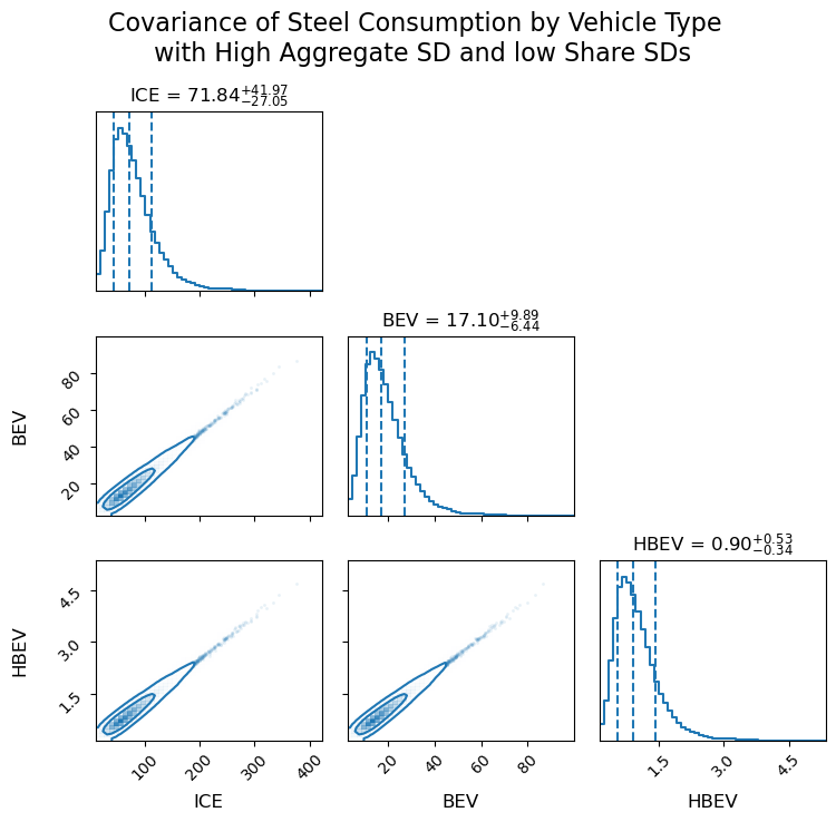
With high uncertainty in the total and low uncertainty in the shares, correlations become positive.
Downstream Analysis: LCA of Carbon Footprint#
Let’s examine how these correlations impact a downstream LCA calculation. We will look at two cases: 1) where the full correlated samples are used in the the down stream analysis (model 2), and 2) where only the summary statistics are communicated from model 1 to model 2.
For simplicity we assume a single emission factor of 2.5 tonnes CO₂ per tonne of steel.
# Set emission factor
emission_factor_steel = 2.5
Approach 1: Using Full Samples (With Correlations)#
Here we assume that researcher 1 has shared the full samples of their model and that these are used by researcher 2:
# Calculate emissions using correlated samples
sample_emissions_full = samples * emission_factor_steel
total_emissions_full = sample_emissions_full.sum(axis=1)

print("Total emissions using the full correlated samples:")
print("Mean emissions:", total_emissions_full.mean(), "tonnes CO₂")
print("SD emissions:", total_emissions_full.std(), "tonnes CO₂")
print("CV emissions:", total_emissions_full.std() / total_emissions_full.mean())
Total emissions using the full correlated samples:
Mean emissions: 250.05792839057565 tonnes CO₂
SD emissions: 7.560662293904017 tonnes CO₂
CV emissions: 0.030235643167029327
Comparing Results with Independent Sampling#
Here we assume that researcher 1 has only shared the summary statistics such as the mean and standard deviation of each sample. We will use two different distributions to sample from: the truncated normal distribution with a lower bound at 0 (naive assumption for the positivity contraint), as well as a gamma distribution as it fits out data better.
from scipy.stats import truncnorm, gamma
means = samples.mean(axis=0)
standard_deviations = samples.std(axis=0)

# Independent sampling ignoring correlations using truncated normal distribution (lower bound at 0)
independent_samples = (truncnorm.rvs(
    loc=means,
    scale=standard_deviations,
    a=(0 - means) / standard_deviations,  # Lower truncation
    b=(np.inf - means) / standard_deviations,  # Upper truncation
    size=(n_samples, len(vehicle_types))
))

# Calculate emissions using independent samples
sample_emissions_independent = independent_samples * emission_factor_steel
total_emissions_independent = sample_emissions_independent.sum(axis=1)

print("Total emissions using the uncorrelated sampling from summary statistics:")
print("Mean emissions (independent):", total_emissions_independent.mean(), "tonnes CO₂")
print("SD emissions (independent):", total_emissions_independent.std(), "tonnes CO₂")
print("CV emissions (independent):", total_emissions_independent.std() / total_emissions_independent.mean())
Total emissions using the uncorrelated sampling from summary statistics:
Mean emissions (independent): 251.0027547084874 tonnes CO₂
SD emissions (independent): 19.41101798021524 tonnes CO₂
CV emissions (independent): 0.07733388425461324
now sample from the Gamma distribution instead#
means = samples.mean(axis=0)
standard_deviations = samples.std(axis=0)

shape = (means ** 2) / (standard_deviations ** 2)
scale = standard_deviations ** 2 / means
# Calculate the shape and scale parameters for the gamma distribution

# Independent sampling ignoring correlations using truncated normal distribution (lower bound at 0)
independent_gamma_samples = (gamma.rvs(
    a=shape,
    scale=scale,
    size=(n_samples, len(vehicle_types))
))

# Calculate emissions using independent samples
gamma_sample_emissions_independent = independent_gamma_samples * emission_factor_steel
total_emissions_independent_gamma = gamma_sample_emissions_independent.sum(axis=1)

print("Total emissions using the uncorrelated gamma sampling from summary statistics:")
print("Mean emissions (gamma independent):", total_emissions_independent_gamma.mean(), "tonnes CO₂")
print("SD emissions (gamma independent):", total_emissions_independent_gamma.std(), "tonnes CO₂")
print("CV emissions (gamma independent):", total_emissions_independent_gamma.std() / total_emissions_independent_gamma.mean())
Total emissions using the uncorrelated gamma sampling from summary statistics:
Mean emissions (gamma independent): 250.47889082546703 tonnes CO₂
SD emissions (gamma independent): 19.455850763489007 tonnes CO₂
CV emissions (gamma independent): 0.07767461241692333
Comparing Distributions#
Let’s compare the uncertainty distributions from both approaches:
import pandas as pd
import seaborn as sns
import matplotlib.pyplot as plt
---------------------------------------------------------------------------
ModuleNotFoundError                       Traceback (most recent call last)
Cell In[14], line 2
      1 import pandas as pd
----> 2 import seaborn as sns
      3 import matplotlib.pyplot as plt

ModuleNotFoundError: No module named 'seaborn'
# Combine results for comparison
comparison_df = pd.DataFrame({
    "Emissions": np.concatenate([total_emissions_full, total_emissions_independent, total_emissions_independent_gamma]),
    "Approach": ["With Correlations"] * len(total_emissions_full) + ["Independent Sampling"] * len(total_emissions_independent) + ["Independent Gamma Sampling"] * len(total_emissions_independent_gamma)
})

# Plot comparison
sns.histplot(data=comparison_df, x="Emissions", hue="Approach", kde=True, bins=50, alpha=0.5)
plt.xlabel("Total Emissions (tonnes CO₂)")
plt.ylabel("Frequency")
plt.title("Impact of Correlations on Uncertainty Estimation (negative correlations)");
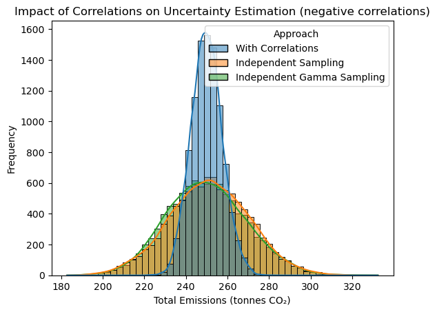
We see that in the case of negative correlations we can overestimate the uncertainty by ignoring the correlations. Now let’s see if we use the experiment with postive correlations:
# Calculate emissions using correlated samples
sample_emissions_full = samples_2 * emission_factor_steel
total_emissions_full = sample_emissions_full.sum(axis=1)

print("Total emissions using the full correlated samples:")
print("Mean emissions:", total_emissions_full.mean(), "tonnes CO₂")
print("SD emissions:", total_emissions_full.std(), "tonnes CO₂")
print("CV emissions:", total_emissions_full.std() / total_emissions_full.mean())

means_2 = samples_2.mean(axis=0)
standard_deviations_2 = samples_2.std(axis=0)

# Independent sampling ignoring correlations using truncated normal distribution (lower bound at 0)
independent_samples = (truncnorm.rvs(
    loc=means_2,
    scale=standard_deviations_2,
    a=(0 - means) / standard_deviations_2,  # Lower truncation
    b=(np.inf - means) / standard_deviations_2,  # Upper truncation
    size=(n_samples, len(vehicle_types))
))

# Calculate emissions using independent samples
sample_emissions_independent = independent_samples * emission_factor_steel
total_emissions_independent = sample_emissions_independent.sum(axis=1)

print("Total emissions using the uncorrelated sampling from summary statistics:")
print("Mean emissions (independent):", total_emissions_independent.mean(), "tonnes CO₂")
print("SD emissions (independent):", total_emissions_independent.std(), "tonnes CO₂")
print("CV emissions (independent):", total_emissions_independent.std() / total_emissions_independent.mean())

# Independent sampling ignoring correlations using truncated normal distribution (lower bound at 0)
shape_2 = (means_2 ** 2) / (standard_deviations_2 ** 2)
scale_2 = standard_deviations_2 ** 2 / means_2
# Calculate the shape and scale parameters for the gamma distribution

independent_gamma_samples = (gamma.rvs(
    a=shape_2,
    scale=scale_2,
    size=(n_samples, len(vehicle_types))
))

# Calculate emissions using independent samples
gamma_sample_emissions_independent = independent_gamma_samples * emission_factor_steel
total_emissions_independent_gamma = gamma_sample_emissions_independent.sum(axis=1)

print("Total emissions using the uncorrelated gamma sampling from summary statistics:")
print("Mean emissions (gamma independent):", total_emissions_independent_gamma.mean(), "tonnes CO₂")
print("SD emissions (gamma independent):", total_emissions_independent_gamma.std(), "tonnes CO₂")
print("CV emissions (gamma independent):", total_emissions_independent_gamma.std() / total_emissions_independent_gamma.mean())

# Combine results for comparison
# Combine results for comparison
comparison_df = pd.DataFrame({
    "Emissions": np.concatenate([total_emissions_full, total_emissions_independent, total_emissions_independent_gamma]),
    "Approach": ["With Correlations"] * len(total_emissions_full) + ["Independent Sampling"] * len(total_emissions_independent) + ["Independent Gamma Sampling"] * len(total_emissions_independent_gamma)
})

# Plot comparison
sns.histplot(data=comparison_df, x="Emissions", hue="Approach", kde=True, bins=50, alpha=0.5)
plt.xlabel("Total Emissions (tonnes CO₂)")
plt.ylabel("Frequency")
plt.title("Impact of Correlations on Uncertainty Estimation (positive correlations)");
Total emissions using the full correlated samples:
Mean emissions: 247.88606853180337 tonnes CO₂
SD emissions: 123.83199965982558 tonnes CO₂
CV emissions: 0.49955207403653723
Total emissions using the uncorrelated sampling from summary statistics:
Mean emissions (independent): 253.4256903708109 tonnes CO₂
SD emissions (independent): 95.76426726694434 tonnes CO₂
CV emissions (independent): 0.377879082135764
Total emissions using the uncorrelated gamma sampling from summary statistics:
Mean emissions (gamma independent): 246.82765372474316 tonnes CO₂
SD emissions (gamma independent): 101.94207503656577 tonnes CO₂
CV emissions (gamma independent): 0.4130091320733833
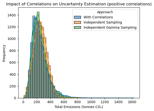
We see from the data and figure above that ignoring positive correlations can lead to underestimation uncertainty in the final result, as well as a (small) bias in the mean value in the case of the truncated normal distribution. That latter result goes to show that one the distribution to sample from is also important: truncated normal distributions have a biased mean and therefore should be used with care!
Conclusion#
The above examples show why considering proper uncertainty propagation including correlation is important in the case of data disaggregation. Ignoring correlations can lead to over-/under-estimation of uncertainty!
The maxent_disaggregation package provides a simple interface for generating statistical samples of disaggregated data while properly accounting for correlations, which is crucial for accurate uncertainty propagation in subsequent analyses.